User Guide
Part IV Analysis and Prediction
EPS China Dada adopts SasS model and provides our users with data processing, visualization, analysis and prediction of high quality, high efficiency and low cost, working as a strong and professional tool for scientific research and academic writing.
In this guide, cases about our analysis and prediction would be presented to help you better understand how to operate on our platform and get the analysis and prediction.
For instance, according to theory and practice, major factors which would influence the output of grain crops include chemical fertilizers, sown area of grain crops, area affected by disasters, total power of agricultural machinery and employed people in the primary industry. With the following steps, such analysis might be achieved.
I. Add Sequence
To begin with, you may get these indicators by way of intra-database search or inter-database search (see Introduction), add these sequence to Cloud Analytics by the function of “Add Sequence”, and create the data set “Grain Crops Production” or select it if you already created one, before you confirm the adding.
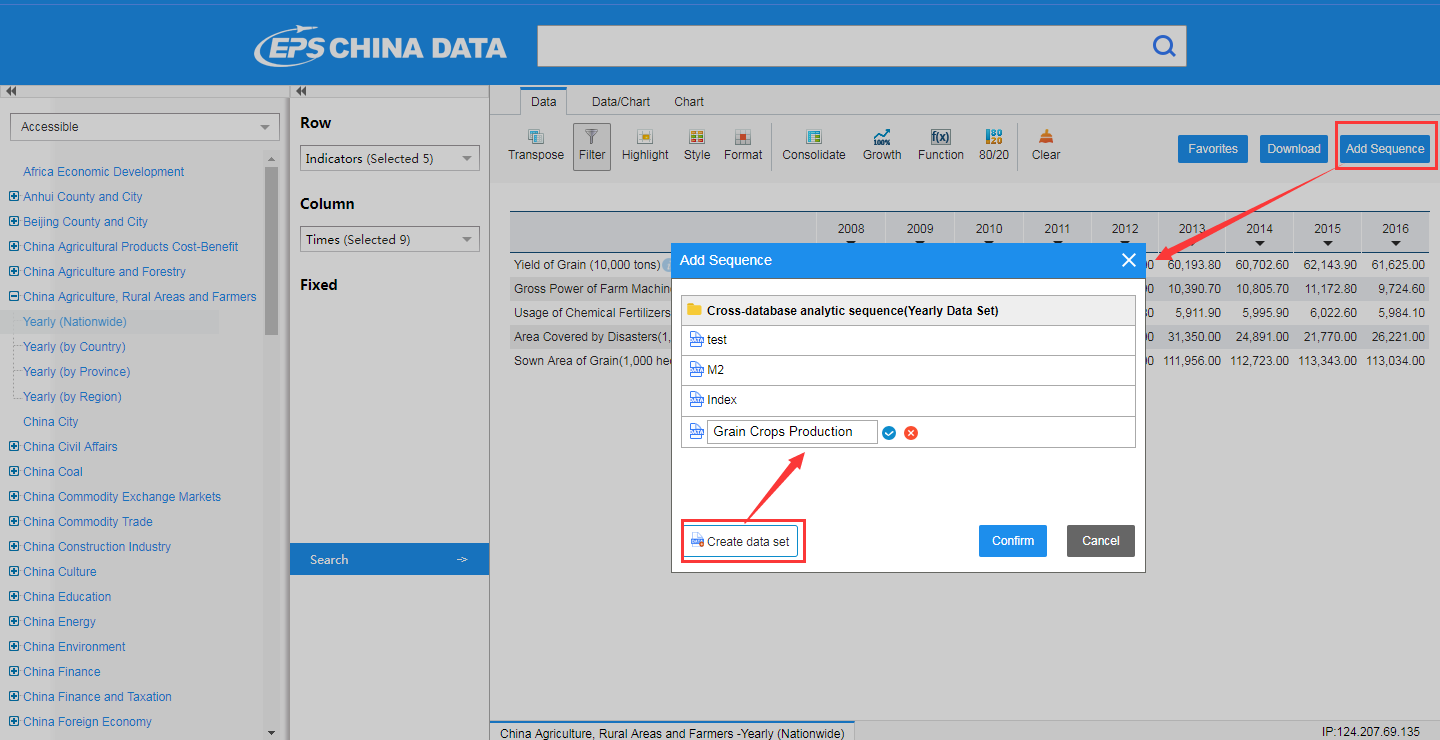
Note: “Add Sequence” is only applicable for data of time series, and for IP login users, please also login My Data Center.
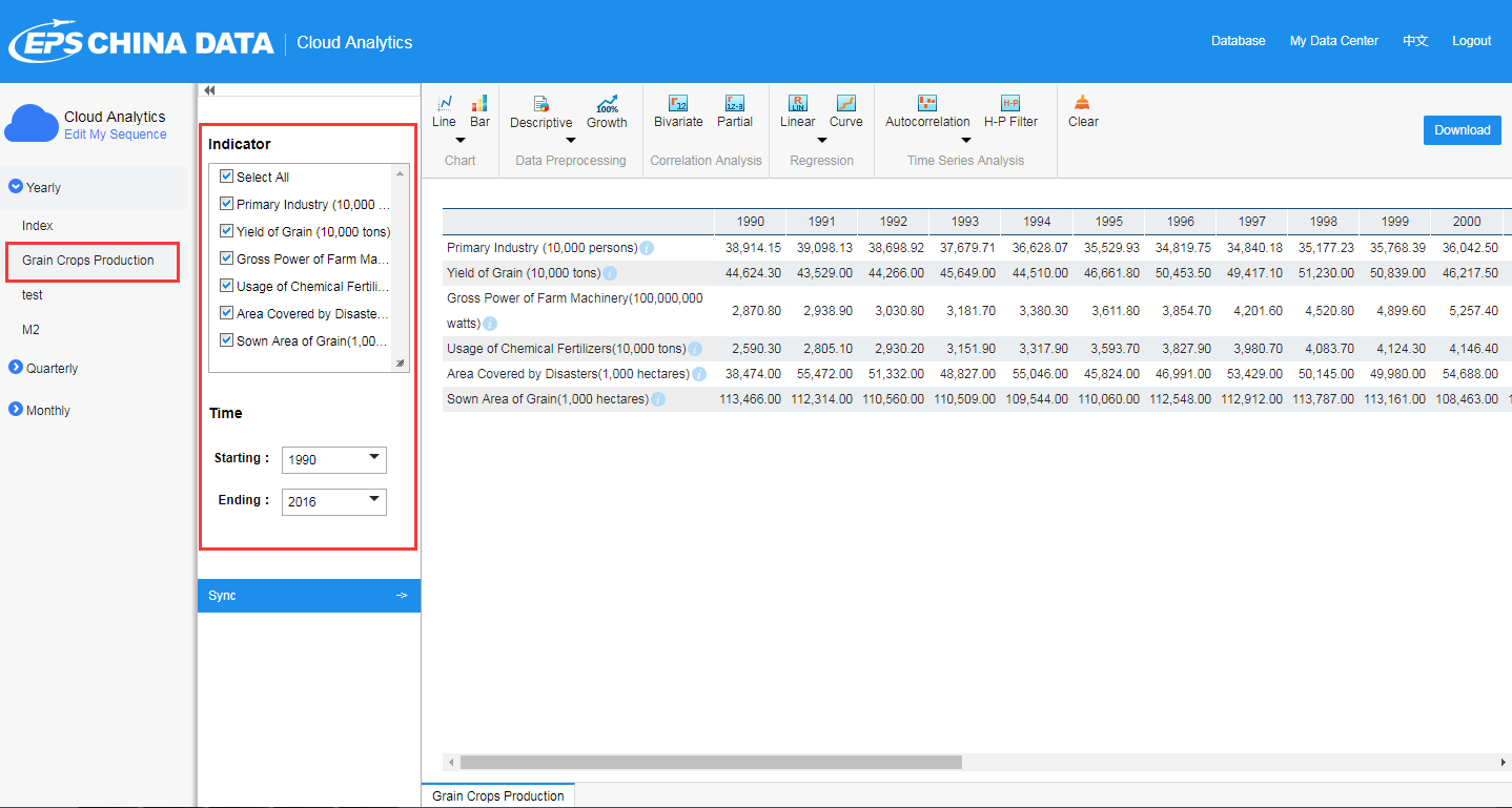
II. Cloud Analytics
Cloud Analytics incorporates functions of charts, data preprocessing, correlation analysis, regression and time series analysis.
In this case, you may enter Cloud Analytics and find the dataset at the left area of the page. From now on you can carry out certain functions.
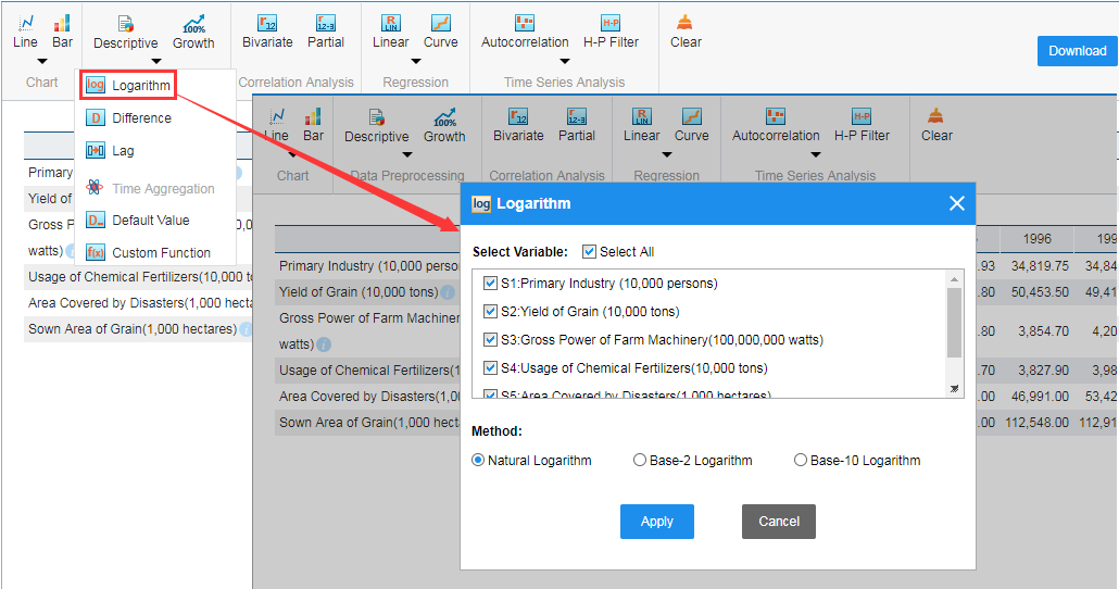
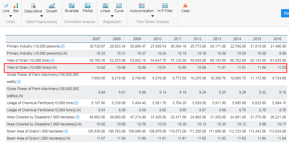
2.1. Data Preprocessing
You may first carry out natural logarithm to all sequences, which could be done by applying Logarithm and select relative parameters.
2.2. Correlation Analysis
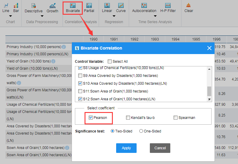
Then you may need to conduct bivariate correlation between variables. For this result, you need to click “Bivariate” and select these sequence preprocessed and other options before you click Apply.
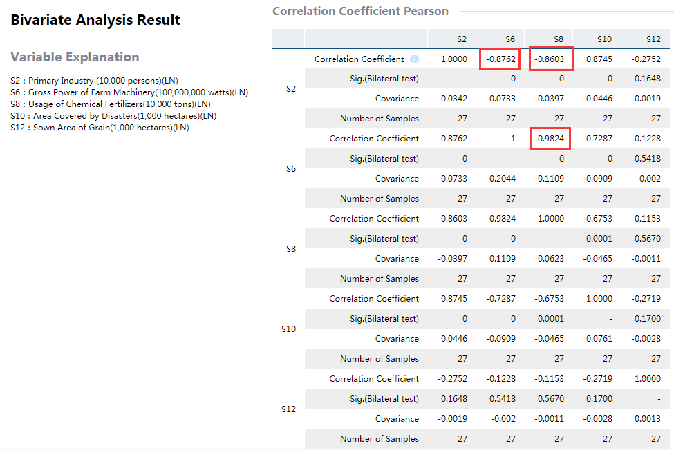
With the result, you can see that there are strong correlations between S2 and S6, S2 and S8, and S6 and S8. Accordingly, a preliminary conclusion may be drawn that multicollinearity exists between S2, S6 and S8, and it might need to take S2 and S6 out from the model.
2.3. Linear Regression
Finally it comes to regression analysis. With the bivariate correlation, you may need to apply linear regression by a click on Linear, and select relative options as follows before you click Apply.
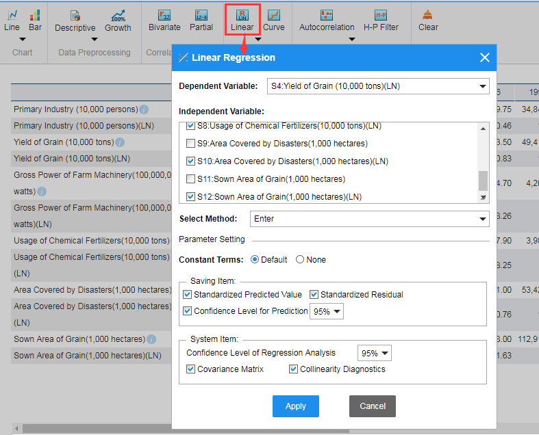
And the result would be as follows,
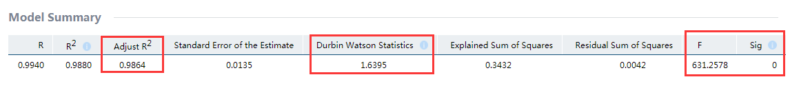
Considering F=631.2578, p<0.05 statistically significant, and the adjusted R-squared =0.9864, it can be seen that there is an overall significant linearity between the output of grain crops and independent variables.
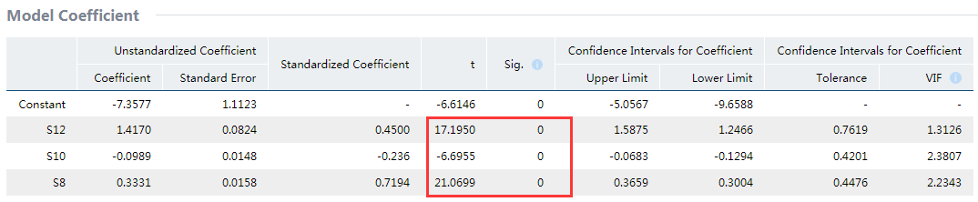
In addition, S8, S10 and S12 have passed Student’s t test.
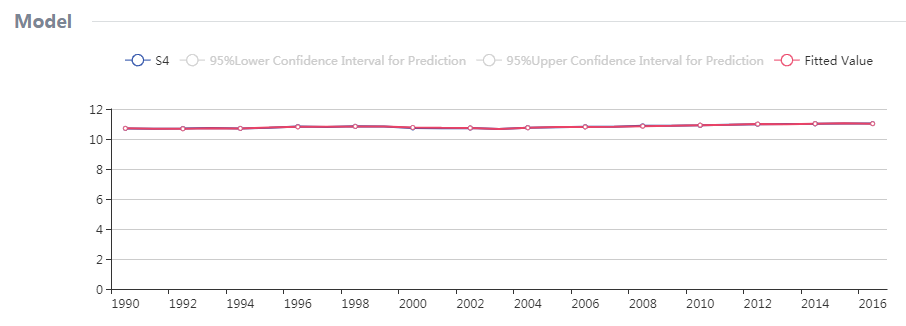
By adjusted R-squared =0.9864, it means the model has good degree of fitting. Besides, the model plot demonstrates that there is minor error between actual value and fitted value.
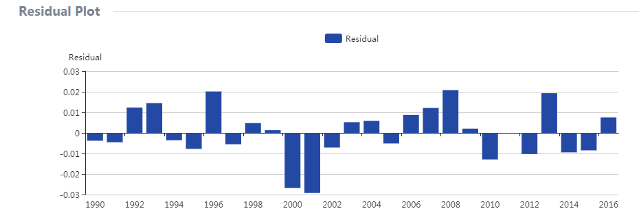
On the other hand, autocorrelation might exist for the residual since this model is built based on time data. However, the residual plot indicates that significant autocorrelation does not occur to the residual sequence.
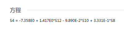
The model expression is
Given the standardized regression coefficient, it can be concluded that utilization of chemical fertilizers and sown area have positive effect on the output of grain crops, which means when other conditions remain unchanged, the higher of the utilization of chemical fertilizers (within a certain range) and the larger of sown area, the higher of the output of grain crops. In addition, utilization of chemical fertilizers has stronger effect than sown are on the output. On the other hand, area affected by disasters has negative correlation with the output, and when other conditions remain unchanged, the larger the area affected by disasters, the lower the output.
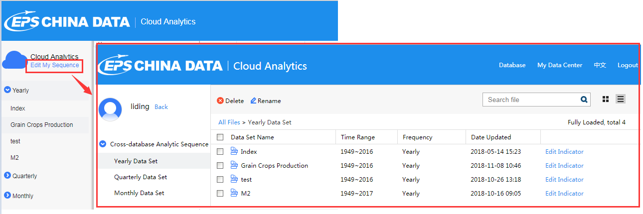
Furthermore, editing function is also available. You may enter Cloud Analytics and click Edit My Sequence on the upper left area of page if you want revise of the data sets or indicators.
Previous Guide: Data Visualization